Understanding pureScale: A Practical Guide to Adoption – Part 1

By Christian Garcia-Arellano and Toby Haynes

Introduction

In the last few years, Db2 pureScale has seen a significant rebirth with its availability in cloud hyperscalers, like AWS and Azure, due to its design that delivers on many of the availability and scalability expectations of cloud environments. Db2 pureScale is the high-end active-active OLTP solution from the IBM Db2 family, and in addition to clouds, it can be deployed in user managed environments on Linux (both RHEL and SLES), on multiple platforms (x86, PPCLe and zLinux), and also AIX environments on Power systems. In short, users choose pureScale because it helps them to reduce the risk and cost associated with growing the compute resources through the implementation of an active-active distributed database solution using the Db2 engine, which enables users to scale dynamically to extreme capacities on demand while maintaining application transparency.

In this blog series we intend to walk you through the process that we have gone over many times with customers looking to adopt pureScale. The goal of this first episode in the series is to take you through some simple steps through the adoption process, that can ensure your application achieves top performance, including using a sound test strategy, and understanding the monitoring tools available to you to identify bottlenecks and be able to apply solutions to each of them. In future installments, we will walk you through some of the simple physical database design considerations, such as indexing, that need to be considered for a successful adoption leaving the application itself untouched and go through several more in-depth performance analysis with their solutions. This is likely not a new topic for the Db2 crowd, as we have had many discussions on the topic since pureScale came to life in 2009, but it is a very good topic for new adopters, and it is always good to refresh everybody on some of the details that we think are necessary for a successful adoption of this powerful technology.

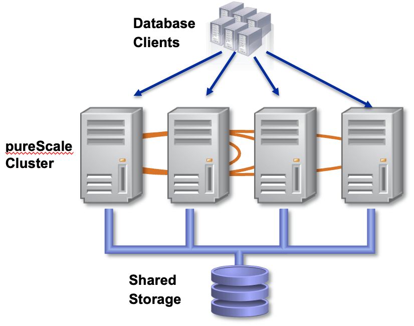
Like we said, we break this first part into two main sections. First, we look at getting ready to move, when you consider some of the basic best practices to get top performance on pureScale, including following a sound test strategy. Then, we look at performance testing your application on pureScale, and what kind of monitoring and tuning techniques can help you reach the performance you want. Note that in this blog we're assuming you're already somewhat familiar with the pureScale architecture, and for this session, we're going to focus on the particulars of moving an OLTP application from a Db2 instance with a single node to a Db2 pureScale instance with an eye to getting the best performance possible. If you want a refresher on the architecture, there is some very good documentation in the Knowledge Center, for example, you can find discussions on the components of a pureScale cluster, deployment options, and cluster topology operations like online add member, drop member, and online add and drop CF. As a quick reminder, you can look at the following diagram, where we show a pureScale cluster in the middle, with multiple members or compute engines, then we show clients connected to those members and being able to run transactions in any of them, and then at the bottom the shared storage component. Of course, in this picture we are missing a key component, the CFs, which provide mainly global locking and global caching to all members to enable the fast data sharing, we will talk about it later on in this blog and subsequent blogs.

Workloads

Let’s start with very basic categorization of workloads, as this is the first important consideration for anybody looking to adopt pureScale.  Most applications destined for pureScale are OLTP in nature, which are characterized by the real-time execution of a large number of concurrent database transactions, for example, coming from banking, finance or retail applications. In fact, usually people thinking of pureScale are thinking of 'enterprise-grade' OLTP, since these need the availability and/or scalability in large measures, the bread and butter of pureScale.  Within these, we then consider the amount of write (INSERT / UPDATE / DELETE) activity in the workload.  The more write activity there is, obviously the more frequently updated the affected database structures are – tables, indexes, metadata, etc.  In the case of pureScale, due to its active-active architecture based on Shared Data, this requires more coordination between members in the pureScale cluster, and can introduce greater chances for contention and bottlenecks that are specific to this technology.

While Db2 pureScale is ideally suited to OLTP workloads, many real-world pureScale deployments have a rich variety of applications connecting to the server. OLAP workloads can be very effective on the pureScale architecture, and modest analytic workloads are also common. It is important that all applications limit the time a transaction is executing, preferably to a few tens of seconds, and applications should be tested to minimize the time spent holding locks. This advice is not pureScale-specific: however, when an application is holding a hot lock on a pureScale cluster it can be delaying transactions on multiple members, effectively serializing the workload. 

We'll find as we go through these installments of the pureScale adoption blog series that we tend to pay more attention to writes (especially INSERTS) than reads. In this regard, it is a good time now to refresh ourselves on the two options of network interconnect available in pureScale environments, TCP and RDMA. This interconnect is a fundamental component in a pureScale cluster, as it is used to communicate between the members and the CFs, so the latency this delivers will have direct impact on the transactional performance a pureScale cluster will provide.  From these two, RDMA is usually a better option for high-write ratio workloads, starting from around 20% writes over 80% reads, due its much lower latency and compute-offset network stack. The duration of the most performance critical operations in pureScale environments, like new lock requests to the CF, are dominated by the network latency in the cluster interconnect. We will get back to this point later on in this first blog, and also later on in the series.

Testing Strategy for pureScale Adoption

The starting point for any pureScale adoption project starts with basic acceptance and functional testing. This is easier than ever with the available deployment options in both AWS and Azure, where you can spin up a pureScale cluster with a TCP/IP interconnect (a.k.a. sockets) in a matter of minutes.  Even without thinking of cloud, it is usually easier to spin up a cluster with TCP than it is with an RDMA interconnect. This is a great starting point as it is always best to have a cluster up and running using components that you likely have on-hand already.  You can even run basic functional tests on one member and one CF if you really need to, the most basic pureScale configuration, and these could be collocated in a single host.  The machine, storage and interconnect requirements for this kind of entry level environments are quite basic – see the Knowledge Center for details – but we highly recommend you look at cloud to get this first phase going in minutes.

To make sure you get great performance on pureScale, some performance and stress test is in order, and ideally you need a sample application that mimics the workload you expect to run in production, covering both operations and data volume.  We know this may not be easy for most, but it is something that will be very useful to have to let you experiment and learn.  Investing in testing can be a powerful tool to accelerate development of production solutions, providing data-driven insights into how database and application changes are interacting in the pureScale environment.

For this next phase, you'll want to make sure your test environment isn’t limited by bottlenecks of its own, such as an under-performing disk I/O subsystem or network interconnect.  Sockets-based interconnect performs well and is sufficient for many uses (smaller clusters with low write ratio and lower transactional rate requirements). It's still best practice to do your performance measurements on a cluster with RDMA interconnect, since that would be our general recommendation for production environments. Here, you'll want at least 2 members and 2 CFs (to support failover tests, etc.), each with 2 or more physical cores and 4 GB to 8 GB of memory per core.

So, in summary:

• Development work and initial 'kicking the tires' functional tests work fine on any kind of pureScale cluster
  • 1-2 small members, 1-2 CFs
  • TCP sockets-based cluster interconnect
  • No particular requirements on CPU capacity, disk performance, etc.
  • Use the smallest (XS) available cloud environments to get this going in no time.

• Performance, scaling and stress testing should be done where there are no artificial resource bottlenecks that would skew the results
  • 2-4 small to medium members, 2 CFs
    • 8 logical CPUs per member & per CF (for example, 4 physical cores on Intel, or 1 physical core on Power).
    • 4-8 GB of memory per logical CPU for members and CFs
  • SAN storage capable of sub-millisecond 4k unbuffered direct I/O disk writes
  • RDMA cluster interconnect is preferable for performance testing, with round trip latency around 30 microseconds (or better). We will discuss this in a subsequent blog in more detail.

Note that in cloud environments, like AWS or Azure, the smallest clusters available are “X-Small”, and those currently deploy 3 members and 2 CFs using c6i.4xlarge EC2 nodes in AWS and F16s V2 on Azure when using TCP/IP transport. In both cases they come with 16 logical CPUs each and 32 GB of RAM. The “X-Small” clusters do not come with bandwidth guarantees and may suffer from network throttling. All other sizes come with a bandwidth minimum of 12.5Gb/s ethernet.

Performance and Scalability Tests with 1 and 2 members

All good scaling tests have a baseline against which you compare 'scaled up' results.  With pureScale, run the workload with a known number of active connections against just 1 member and make that your baseline for comparisons to test with more members. That way, as you add a 2nd and maybe a 3rd or 4th member, you can plot the growth in cluster throughput against the 1-member baseline. Standard practice is to double the number of active connections to the pureScale server as you double the number of pureScale members.

You can compare your test workload throughput on the pureScale cluster against another system – for example, a separate Db2 instance with a single node system – but it's often the case that the hardware configuration of the single node system differs from what you're using for pureScale, in terms of CPU, memory, storage, etc.  This can inject uncertainty and 'noise' into your comparisons, since it can be hard to predict how much impact these underlying differences might have on their own.   Even if you bring a non-pureScale result into the equation for comparison with the overall cluster, you should still run 1 member tests on pureScale to measure scalability.

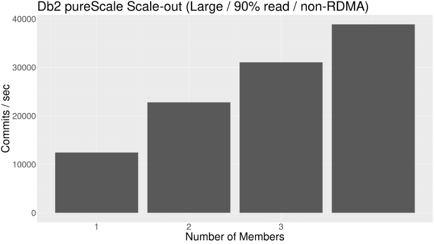
Scaling up from 1 to 2 members can tell you a lot about how your application is going to perform on pureScale, and this is a good predictor of how things will go as more members are added.   In terms of cluster capacity – how much total work can you get done – it's worthwhile to also consider going to 4 members if you can, as a very common deployment configuration. The following chart shows the scalability we observed using a typical transactional workload. This is running in an AWS environment, and using a 90/10 read/write ratio.

Monitoring

Db2 pureScale has the same basic types of resource requirements as non-pureScale, that is, adequate CPU, memory, disk and client network capacity.  Monitoring these is done the same way in pureScale as non-pureScale, and is not really the topic of this blog, so for now we're going to assume that these are under control, as we are assuming you have a current system that is non-pureScale to compare with. As a result, we'll focus more on the tools that allow you to identify the potential cluster-specific issues you might run into, and how to detect and resolve them. Having said this, we expect that you would continue to monitor these basic metrics, as CPU consumption or IO consumption can vary as changes are made to the workload or the configuration.

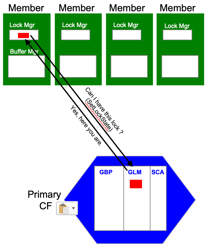
Before we dig in to the tools specific to pureScale, let’s just do a quick review of the potential issues that you may find given that pureScale introduces a brand-new component, the Cluster Caching Facility (CF) that serves as the cluster coordinator to manage the data sharing functionality and make your pureScale environment perform. First, the CF provides a Global Lock Manager (GLM), and we'll look at the tools to identify possible cross-member lock contention. The most important function the GLM provides is granting locks, and for this members invoke a SetLockState operation. Setting a lock state on the CF is a quick operation (around a microsecond), so the lower the network latency, the faster these lock requests from the members will be completed, reducing the impact on transaction processing. If you want to dig further into these, and have a pureScale cluster handy, have a look at the MON_GET_CF_CMD monitoring function. In there you will see the times for each CF operation, including SetLockState. This diagram shows this kind of operation in progress. This is usually what is involved for a lock that is currently free, but when a lock is being held by another member, the operation is more involved because it may require a lock negotiation to free the lock before the lock request is granted. Here is a diagram that shows the basic flow of a lock request:

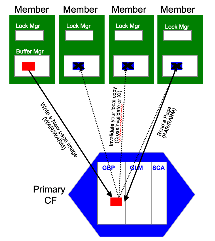
Second, pureScale introduces a cluster-level Group Buffer Pool (GBP) in the CF, and we'll want to make sure it's performing well and being effective. Two of the most common operations in the GBP are writes and reads of pages. In the case of write to update a page in the global cache, driven by the WriteAndRegister APIs (WAR, or WARM), in turn could drive cross-invalidations or XIs to all members that have a copy of these pages in their local cache, as those become stale and should not be used anymore. Once all XIs complete, the CF will respond to the member with the completion of the WAR/WARM operation. Here is a diagram that shows this basic flow:

You can also see all of these in the MON_GET_CF_CMD monitoring output as well, and you will see once we dig into specific analysis that this becomes a very important piece of diagnostics, we will look at it over and over. The other thing useful to add here is that CrossInvalidate, or XIs, given that they carry very minimal payload, they are a good operation to look at when trying to validate network latency.

As you can imagine, given that the communication between members and CFs is one of the key differences moving to a pureScale cluster from a standalone Db2 or Db2 HADR configuration, we'll look at how to monitor it to identify bottlenecks that might develop in the cluster interconnect under heavy load. Finally, we'll also consider ways to balance load across the cluster.

MONREPORT.DBSUMMARY()

The easiest way to monitor Db2 pureScale metrics is with our old friend, MONREPORT.DBSUMMARY.  If you're not familiar with it, this is a stored procedure which returns a nice, easy-to-read text report of key performance metrics.  DBSUMMARY() superceeds 'snapshot for database', and includes metrics which aren't in snapshots, such as a few very helpful ones which are specific to pureScale. Monitoring in pureScale typically goes one of two ways – either specific to the member you're connected to (good for host-specific diagnostics) or for the cluster as a whole (which is a good way to start out). MONREPORT.DBSUMMARY() takes the latter approach, reporting information for all cluster members, rolled together. Conveniently, MONREPORT.DBSUMMARY() reports activity just for the interval we measured (e.g. 30 seconds, based on the input parameter) rather than the cumulative counts and times since database activation that the monitor functions track by default. This saves us the trouble of sampling twice and finding the delta values.

This tool gives us insights into workload volume at the database-level scope. For example, you can see the number of commits and activities per second, like the following:

Work volume and throughput

-----------------------------------------------------

                          Per second     Total                 

                          -------------  ------------

TOTAL_APP_COMMITS         708            42539

ACT_COMPLETED_TOTAL       70902          4254128

APP_RQSTS_COMPLETED_TOTAL 74448          4466920

Another useful set of data are the times spent doing certain specific things, like compiling, or sorting. DBSUMMARY() also summarises the wait times, for example waiting for the CF or disk I/O, which in pureScale environment is critical to understand, especially when comparing with a non-pureScale environment running the same workload. Like we said, these provide a cluster-level view to get an idea of where the bottlenecks may be, but to understand the detail you need a more detailed report, which is what db2mon does, and we describe in the next section.

-- Wait time as a percentage of elapsed time --

               %   Wait_time/Total_time

               --- ----------------------------------

For_requests   72  4822949/6615608

For_activities 71  3246460/4515606

-- Detailed breakdown of TOTAL_WAIT_TIME --

                     %    Total

                     ---  ----------------------------

TOTAL_WAIT_TIME      100  4822949

I/O wait time

  POOL_READ_TIME     16   795423

  ...

  LOG_DISK_WAIT_TIME 3    184917

LOCK_WAIT_TIME       0    0

...

CF_WAIT_TIME         58   2825874

db2mon

The tool that we use extensively is db2mon, as evidenced in recent presentations and blogs. The db2mon script is the “go-to” tool when trying to diagnose performance behavior because it is more comprehensive, light weight and powerful. This tool leverages the existing SQL monitoring interfaces and can collect all of the necessary elements to perform an in-depth report of the performance at that point in time, per member and at multiple levels of scope (database-wide, connection, SQL statement and more).

When db2mon is run, it will collect the monitoring metrics for a set amount of time and will generate a detailed report section as the output. Since this is a well-known tool that has been available for many years, and it is documented in the Knowledge Center, we are not going to go into a lot of detail into how to use it, and we ask the reader to refer to either the blog written by Kostas Rakopolous with everything you want to know about db2mon, and also refer to the youtube video with an introduction to the tool in under 45 minutes.  

Throughout the rest of the series we are going to use this tool extensively to show the kind of analysis that we need to do to diagnose the issues that you can encounter. These analyses often include some of the specific metrics reported by the tool that are pureScale-specific, like CF#RTTIM, which reports the round-trip CF command execution counts and average response times. We mentioned this being useful before when we were talking about SetLockState using MON_GET_CF_CMD, which is what db2mon is using to collect these diagnostics and produce the report. Another example of a pureScale specific section is CF#GBPHR, which reports Group buffer pool data and index hit ratios, which can be analyzed together with BPL#HITRA for local buffer pool data and index hit ratios to understand the interactions between the global cache and the local caches.  

Conclusion

In this first blog entry, we’ve outlined our initial approach to moving applications to Db2 pureScale. We’ve discussed the types of workloads that are most suited to pureScale (OLTP or OLTP-like, with shorter transaction times), the importance of test workloads and a brief introduction and how to monitor those workloads with existing tools provided as part of Db2 pureScale. 

In the upcoming blog posts, we will go much further in looking at database design, database schema and objects, and how to obtain insights into the workloads to understand the performance of the application across the pureScale cluster.

About the Authors

Christian Garcia-Arellano is STSM and Db2 OLTP Architect at the IBM Toronto Lab, and has a MSc in Computer Science from the University of Toronto. Christian has been working in various DB2 Kernel development areas since 2001. Initially Christian worked on the development of the self tuning memory manager (STMM) and led various of the high availability features for DB2 pureScale that make it the industry leading database in availability. More recently, Christian was one of the architects for Db2 Event Store, and the leading architect of the Native Cloud Object Storage feature in Db2 Warehouse. Christian can be reached at cmgarcia@ca.ibm.com.

Toby Haynes has a background in Observational Astronomy at the University of Cambridge, England.  Toby joined IBM Canada in 1999 as a software developer in the Db2 Runtime engine. After eight years of development experience, he moved over to the Db2 Performance team to start work on what would become Db2 pureScale v9.8, working under Steve Rees. In the late summer of 2018, he stepped up to the role of Technical Manager for Db2 pureScale, looking after an active team of developers and support analysts. Now a Senior Software Developer and Program Owner for Db2 High Availability at IBM, Toby is looking forward to taking Db2 pureScale forward to new opportunities.