AI Vectors and Similarity Search - A Gentle Introduction

IBM Db2 has introduced a native vector data type and vector similarity search capabilities in its latest Early Access Program (EAP) release. These new features enable Db2 to support powerful AI-driven use cases such as semantic search, recommendations, and Retrieval-Augmented Generation (RAG) for large language models (LLMs).

In this post, we’ll cover the fundamentals of vectors and vector similarity search—providing the background you need to understand these new capabilities and their role in powering modern AI applications. Whether you’re new to this topic or just looking for a refresher, this article will walk you through the core concepts of vectors. For details specific to Db2’s vector features, be sure to check out the EAP release notes.

What Is a Vector?

A vector is an ordered list of numbers that represents data in a mathematical form. In programming terms, it’s similar to an array or list of numeric values—like a = [1, 2, 3, 4]. Each number corresponds to a specific dimension or feature of the data.

What makes vectors valuable is their ability to encode complex information, allowing mathematical operations such as measuring distance or similarity. This capability is fundamental in many applications, from comparing text and images to matching user preferences or product features.

Why Are Vectors Important?

Vectors provide a way to represent complex, non-numeric data—such as text, images, audio, and user interactions—in a structured numerical format that algorithms can easily process. By converting data into vectors, we enable mathematical operations like calculating distances and similarities between data points, which are fundamental to many machine learning and AI tasks.

For example, consider the challenge of comparing three words: apple, banana, and computer. Instinctively, we recognize that apple and banana are more closely related—they’re both fruits, edible, and naturally grouped together in our minds. In contrast, computer belongs to a different category—electronics—with distinct attributes and purposes. While these associations come naturally to us, teaching machines to understand and compute such relationships is far more complex. This is where vectors and vector similarity search come into play. 

Which pair of words is more closely related: apple, computer, or banana?

For apple, computer, and banana, I got their vector representations using word2vec-google-news-300, a pre-trained model developed at Google in 2013 for generating vector representations for words. This model was trained on approximately 100 billion words from the Google News dataset and contains 300-dimensional vectors for 3 million words and phrases. ​

To enrich the visualization, which I will present shortly, and provide more data points in the vector space, I expanded the initial list to include additional words:

• Fruits: apple, banana, pears, grape
• Electronics: phone, computer, tv, remote
• Furniture: chair, table, sofa

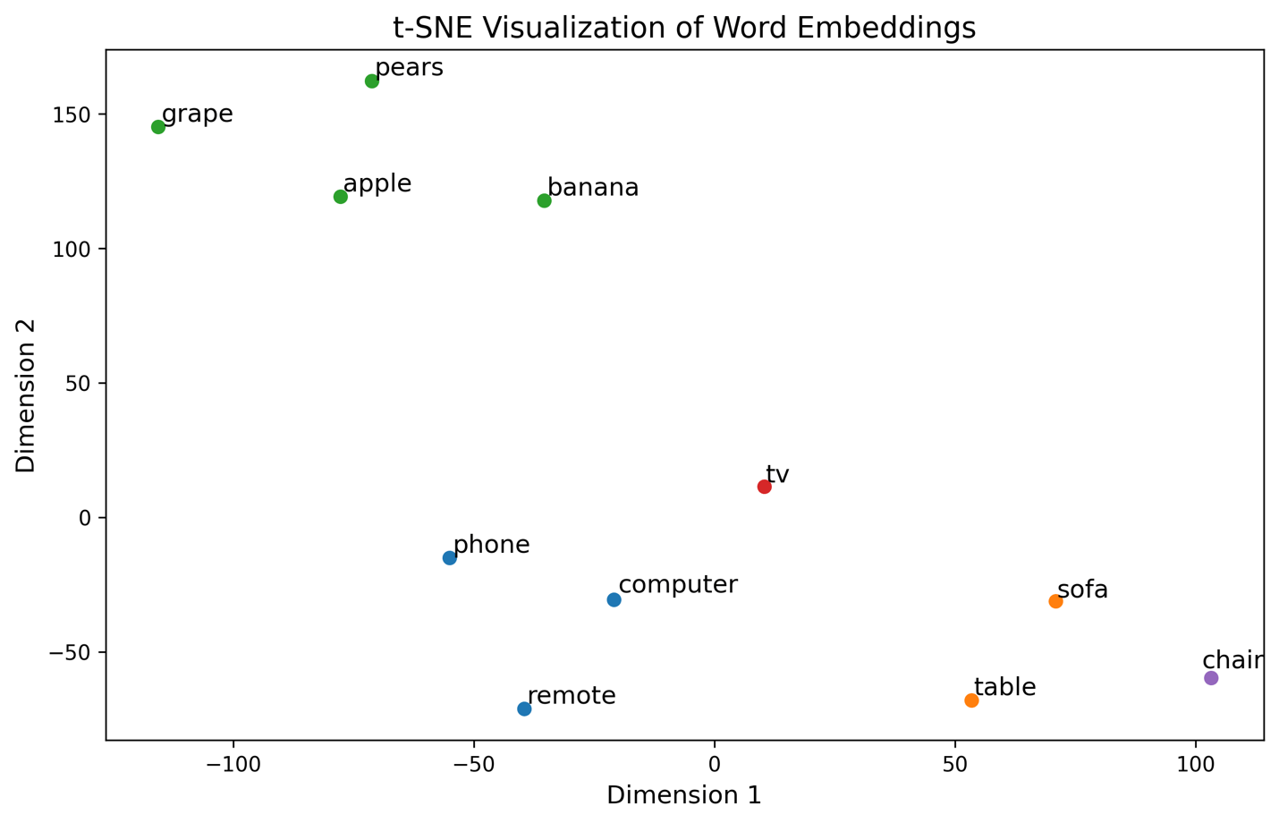
Next, I applied t-Distributed Stochastic Neighbor Embedding (t-SNE)_[1], a widely used technique for reducing high-dimensional data to lower dimensions, to visualize the above word vectors in a two-dimensional space. t-SNE is particularly effective for visualizing complex datasets by preserving local structures and revealing patterns within the data.

The following t-SNE visualization of a learned vector space shows how words like fruits, furniture, and electronic devices are grouped based on their similarities. Fruits like apple, banana, grape, and pears cluster together due to shared traits like being edible and related to food. Electronic devices such as computer, phone, remote, and TV form a separate group, highlighting their functional differences. Furniture items like sofa, table, and chair are grouped together, showing their closeness as household items. The positioning of words in the plot allows for mathematical differentiation between unrelated categories.

Using such learned vector representations on a vector space, applications can:

• Discover relevant items even when different words or phrases are used in describing them.
• Differentiate between meanings based on context (e.g., Apple the company vs. apple the fruit).
• Power applications such as semantic search, recommendation systems, and RAG.

For example, a search for "healthy snacks" might prioritize apple, banana, and pears based on vector proximity—even if the query doesn’t mention these fruits directly. Similarly, a search for "home entertainment devices" would pull tv, remote, phone, and computer, bypassing unrelated categories like furniture or fruit.

Once data points are transformed into vectors using a consistent scheme, we can measure how closely related they are. Words with similar meanings or that belong to the same category naturally map to a region closer in a vector space. This ability to quantify similarity is essential in applications like semantic search, recommendation systems, and natural language processing. Instead of relying on exact matches, systems can retrieve relevant results based on meaning and context—enabling smarter, more intuitive experiences across a wide range of real-world scenarios.

Embedding: Turning Data Into Vectors

Embedding is the process of converting raw data—such as text, images, or audio—into numeric vectors. Specialized AI models, called embedding models, learn patterns and relationships within their training data and map similar data points close together in high-dimensional vector space.​ Training embedding models from scratch is often costly and resource-intensive due to the need for large datasets and significant computational power. To address this, pre-trained embedding models are commonly used to convert various data types—such as text, images, and audio—into vector representations. New models continue to emerge regularly, expanding the possibilities for generating high-quality embeddings. These models, trained on extensive datasets, capture intricate patterns and relationships within the data, enabling effective feature extraction for downstream tasks.​

For instance, in natural language processing, models like Word2Vec (2013) and GloVe (2014) generate word embeddings that encapsulate semantic relationships between words. Similarly, in computer vision, models like ResNet (2015) produce image embeddings that capture visual features. The vector representations produced by these embedding models are known as embedding vectors, which serve as numerical representations of the original data, facilitating various machine learning and AI applications.

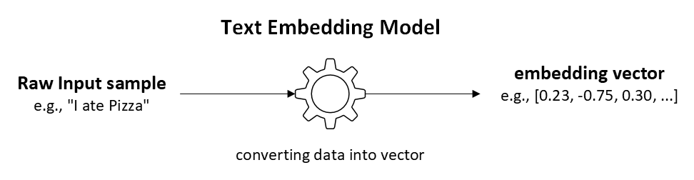
Text Embedding Models convert words, sentences, or documents into vectors that capture semantic meaning. Text embedding models have token limits and fixed vector dimensions. Various LLM service providers offer different embedding models. For example, IBM’s watsonx.ai platform has a range of text embedding models with specific token limits and vector dimensions. It’s important to select an embedding model that fits your application’s needs, considering factors like token limits, vector dimensions, and compatibility with your LLM service provider. 

[Source: Supported encoder foundation models in watsonx.ai]

These models can be accessed via the watsonx.ai API for tasks such as semantic search, document comparison, and retrieval-augmented generation (RAG). The widespread adoption of pre-trained embedding models has led to significant improvements in various applications, including recommendation systems, search engines, and conversational AI, by providing quick and efficient ways to represent complex data.

Measuring Vector Similarity

After converting data points into vectors, we can compute the similarity between pairs of vectors within the vector space. This comparison helps determine how closely related two data points are based on their vector representations. Vector similarity is typically measured by calculating the distance between two vectors in the space. It’s important to note that both vectors must have the same dimensions for these calculations to be valid.

Several distance metrics are available for comparing vectors, each with its own strengths and suitable use cases. Commonly used metrics include Euclidean distance, cosine similarity, dot product, Hamming distance, and Manhattan distance. These metrics help quantify similarity or difference between vectors, enabling various AI and machine learning tasks such as search, recommendation, and classification. 

Below, I briefly describe each of these distance metrics.

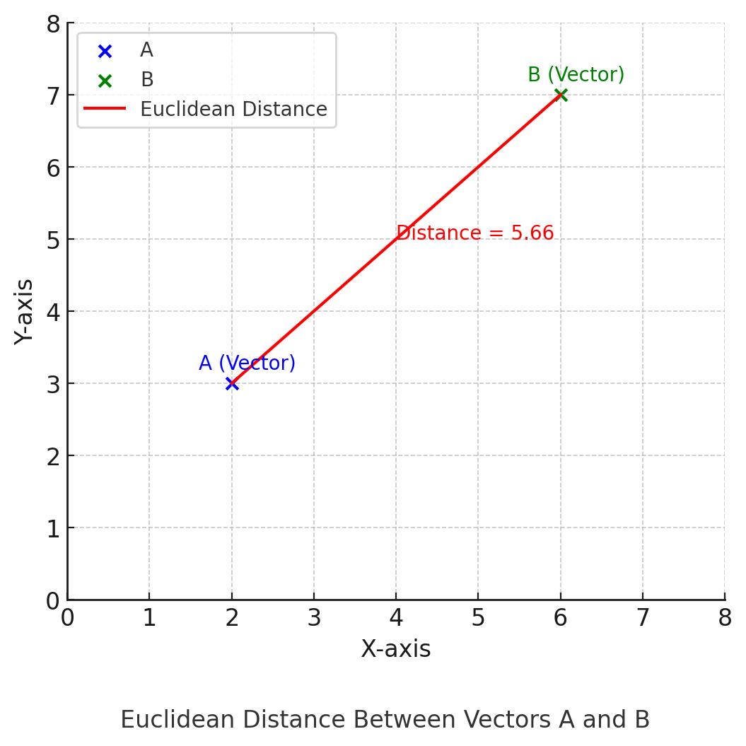
Euclidean Distance

Euclidean distance measures straight-line distance between a pair of points in the Euclidean space. It's measured as follows:

L2 distance(A, B) = √∑_i (A_i - B_i)²,

where A and B are two vectors and A_i and B_i are individual vector coordinates. 

The following plot visualizes the Euclidean distance between two vectors, A (blue) and B (green), represented as points in 2D space. The red line shows the straight-line distance between the two vector endpoints, illustrating how Euclidean distance measures similarity based on spatial proximity. The distance value is labeled along the line, providing a geometric interpretation of how far apart the two vectors are in vector space.

Since Euclidean distance is a dissimilarity measure (larger value = less similar), the interpretation works inversely:

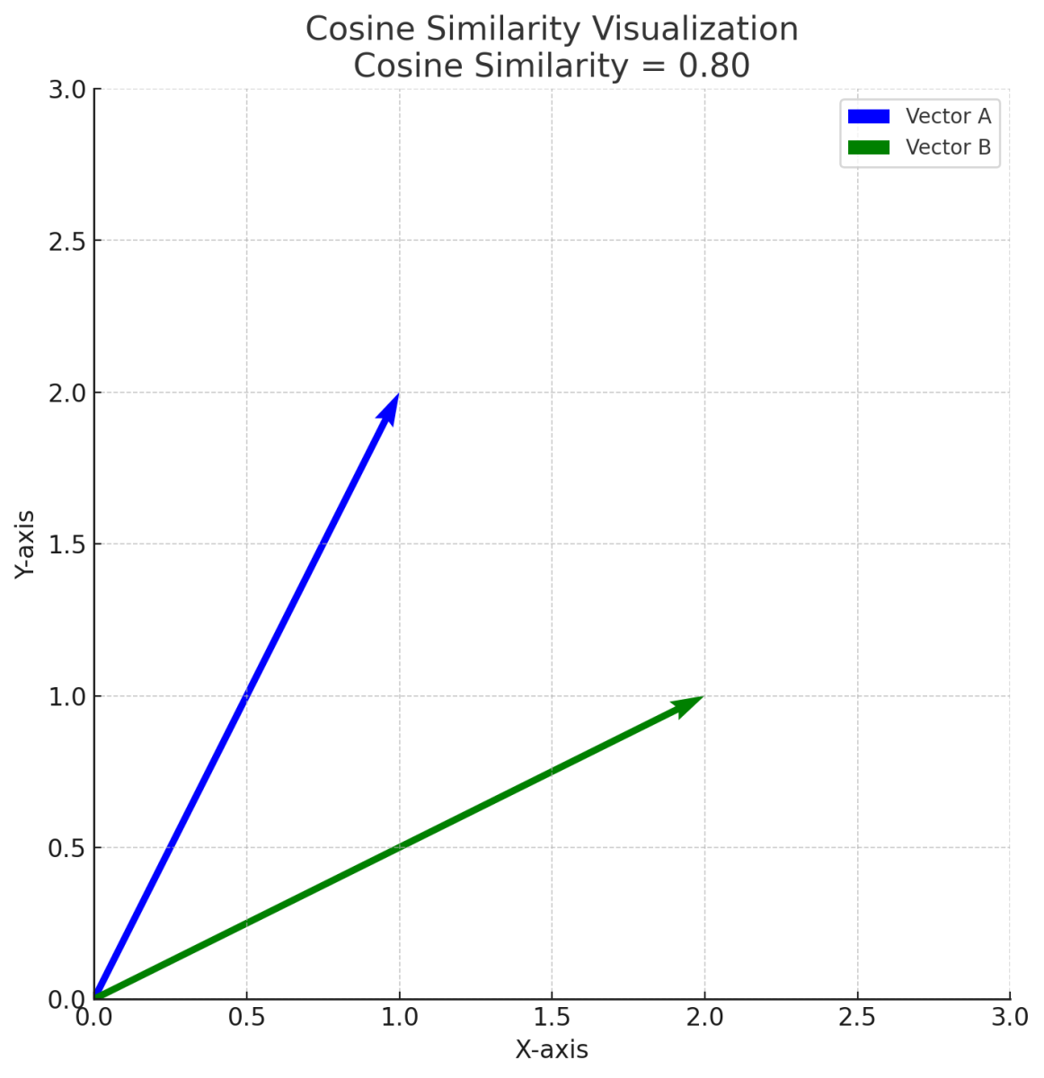
Cosine Similarity

Cosine similarity measures the angle between a pair of vectors, focusing on direction rather than magnitude. It uses the following formula:

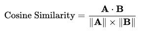
Where 

• A . B is the dot product of vectors A and B
• || A || is the magnitude (norm) of vector A
• || B || is the magnitude (norm) of vector B

The following plot visualizes cosine similarity between two vectors A (blue) and B (green). The angle between the vectors represents their similarity — the smaller the angle, the higher the cosine similarity. In this example, the calculated cosine similarity is approximately 0.80. Cosine similarity measures the angle-based similarity between vectors, independent of their magnitudes.

While the theoretical range of cosine similarity is -1 to 1, the nature of data in many practical applications restricts this range to 0 to 1. For instance, when comparing a pair of documents, you would compute their degree of similarity, but not if one document is opposite to the other. This reflects varying degrees of similarity, from no similarity (0) to complete similarity (1). When two vectors point in exactly the same direction, the angle (θ) between them is 0 degrees. The cosine of 0 degrees is 1, resulting in a cosine similarity of 1. ​ This indicates maximum similarity, meaning the vectors are perfectly aligned.

Cosine similarity is not a distance—it’s a similarity score. However, some applications compute cosine distance as:

Cosine Distance=1−Cosine Similarity

Manhattan distance

For a pair of vectors, Manhattan distance sums the absolute differences across each dimension. It's computed as follows: Manhattan Distance

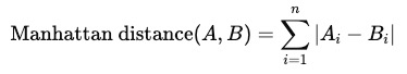
Where:

• A and B are two vectors of the same dimension
• n is the number of dimensions
• |A_i - B_i| is the absolute difference between the components of vectors A and B

Manhattan distance calculates the distance traveled on a grid, similar to a taxi moving through city blocks, hence the name “taxicab” distance.

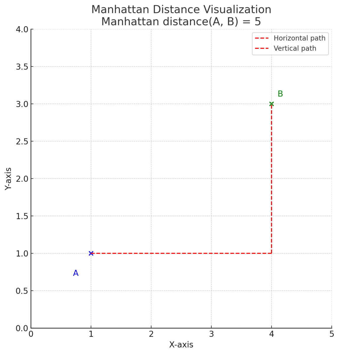
The above plot shows Manhattan distance (A, B) between two points. Red dashed lines represent city block path - first horizontally, then vertically. Total length of this path equals Manhattan distance.

Hamming Distance

Hamming distance counts the number of dimensions in which two vectors are different. It's usually used when comparing a pair of binary vectors - i.e. where vector elements are 1s and 0s. 

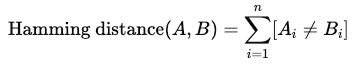
Where:

• A and B are vectors of the same dimension
• n is the total number of dimensions
• [A_i ≠ B_i] is 1 if the value at position is different, 0 if they are the same

Consider the following 2 vectors: 

• A: [1, 0, 1, 1, 0, 1]
• B: [1, 1, 1, 0, 0, 0]

The following table compares the element-wise comparison between A and B:

In dimensions, 2, 4, and 6, A and B vectors differ. So, their hamming distance is 3. 

Tasks such as error detection, DNA sequence comparison, and binary feature matching frequently use hamming distance.

Dot Product

The dot product is a similarity metric that measures how well two vectors are aligned. It is calculated by multiplying the corresponding components of the two vectors and then summing the results. A larger dot product indicates higher similarity (strong alignment), while a smaller or negative value indicates less similarity.

The formula is:

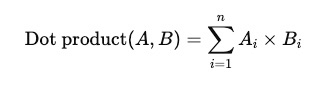
Where:

• A and B are vectors of the same dimension
• A_i and B_i are the values at dimension i
  
  

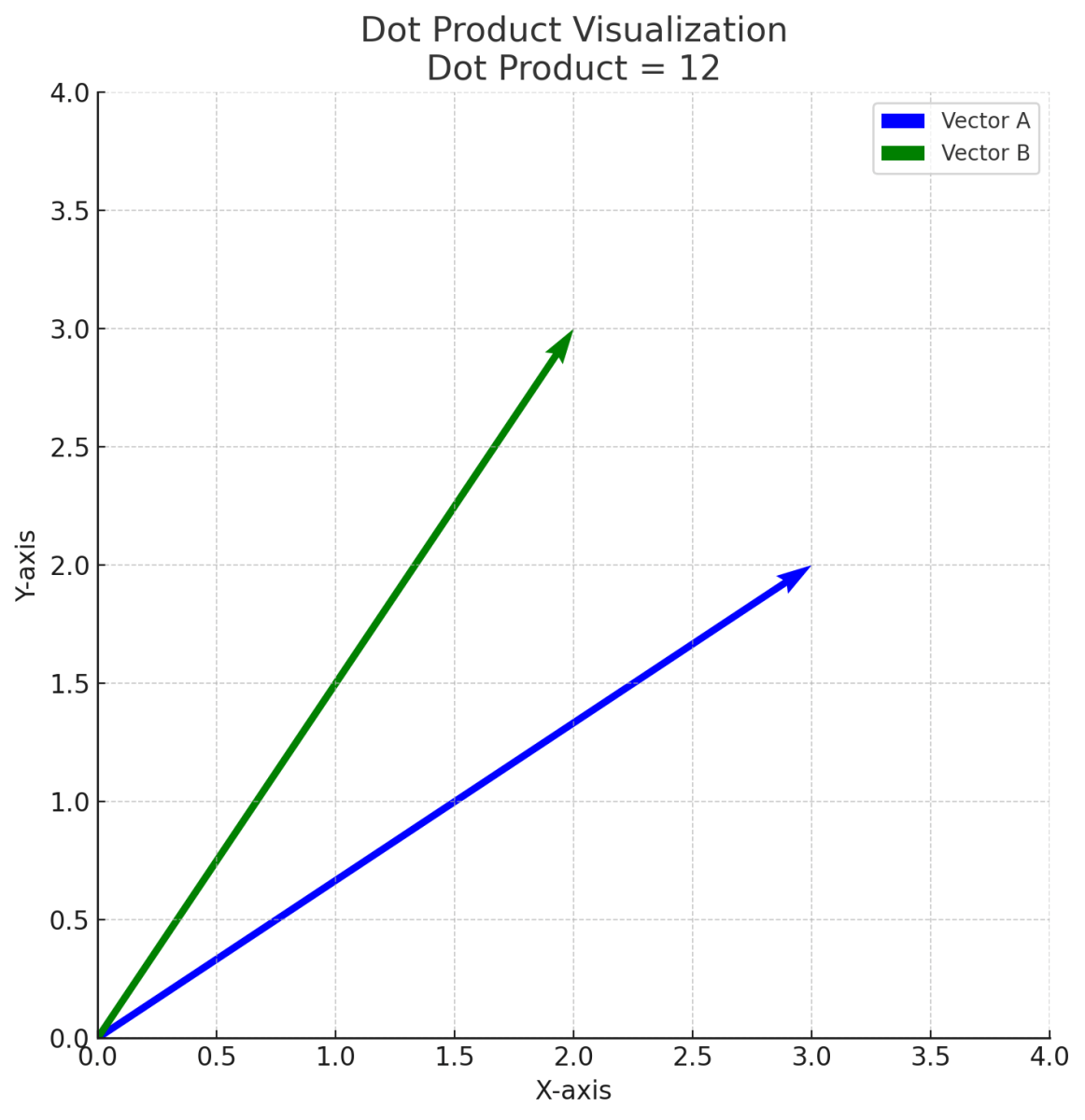
The above plot shows an example dot product similarity between two vectors A (blue) and B (green):

• The angle and alignment between the vectors affect the dot product.
• A larger dot product means that the vectors are somewhat aligned in direction.
• If vectors point in opposite directions, their dot product would be negative
• when the angle between vectors is 90°, their dot product would be zero.

The dot product is a measure of similarity between two vectors, indicating how closely they align in direction. However, it can be transformed into a distance metric, which quantifies dissimilarity, by applying specific adjustments.

Distance=−(A⋅B)

This negative dot product ensures that:​

• Vectors with a higher dot product (more similar) yield a smaller (more negative) distance.​
• Vectors with a lower or negative dot product (less similar) yield a larger (less negative or positive) distance.

Consider the following 2 vectors:

A = [1, 2, 3] and B = [4, 5, 6]

Dot product, A⋅B=(1×4)+(2×5)+(3×6)=4+10+18=32

Distance =−32

Here, negative, thus smaller, distance is higher similarity.

Final Thoughts

Vectors and vector similarity search are revolutionizing how we process complex data in AI and search technologies. When we convert data into numerical form, we empower machines to assess similarity, reveal patterns, and provide more intelligent outcomes—such as suggesting a movie, finding the correct document, or enhancing the responses of AI models. Grasping these ideas is an important initial stride in unleashing the capabilities of contemporary AI-driven systems.

References

[1] Van der Maaten, Laurens, and Geoffrey Hinton. "Visualizing data using t-SNE." Journal of machine learning research 9, no. 11 (2008).