The Neural Networks Powering the Db2 AI Query Optimizer
Sceptical about anyone trying to tell you your database system's query optimizer needs AI? Read this1. Still don't think AI or ML can help generate better SQL access plans for improved query performance? Read that2.
Some say the query optimizer can be thought of as the brain of your database management system. How is it possible to integrate neural networks into a highly sophisticated query optimizer? It wasn't exactly brain surgery.... although maybe in a way it was? Read on to find out more.
A strong background in Machine Learning is not required as AI/ML concepts in this article are introduced at a high level. Most low-level technical details, although critical to ensure models are trained and function properly to yield optimal results, are intentionally omitted in order to focus on a higher-level conceptual understanding of the Db2 AI Query Optimizer.
Overview of Neural Networks used by the Db2 AI Query Optimizer
The AI Query Optimizer uses a separate neural network for each table enabled for AI query optimization. Neural network layers allow for hierarchical feature extraction, where each layer in the network progressively refines the representation of the input data 3. Neural network learning (using back-propagation of error) helps the network learn the features to optimize a specific task. In our case the inputs are representations of the query predicates for columns in a table, and the task to be optimized is selectivity determination of those query predicates. At a high level, you can think of this feature extraction as a way to learn the characteristics of the underlying data (e.g. such as how data from various columns is correlated), and after these features have been learned during model training, using them to better predict the selectivity from a given set of input column predicates. This selectivity can then be converted into a cardinality estimate by multiplying the table cardinality (the number of rows in the table), and used by the query optimizer to determine the most optimal access plan to use for a particular query. Conceptually, optimal access plans are typically ones that apply the most selective or restrictive predicates first, reducing the number of rows that need to be evaluated by other predicates, and the rows that need to be processed by other operators such as hash joins or sorts. Using AI to improve cardinality estimates helps the optimizer determine more optimal query access plans.
How are the Neural Networks Trained?
How exactly though can these neural networks be trained to learn the underlying data correlations between the various columns?
The neural networks are trained using supervised learning, which means they learn from a training set that includes both input features (i.e. encoded column predicates similar to those that may be specified in a SQL query), as well as the expected query selectivity that should result from running a query containing those column predicates. So, we first need some way of generating a representative training set. For this, we rely on the existing Db2 automatic statistics collection facility, which gathers table and column statistical information that has been crucial for the functioning of the traditional Db2 statistics-based query optimizer.
Automatic Statistics Collection Table Sample
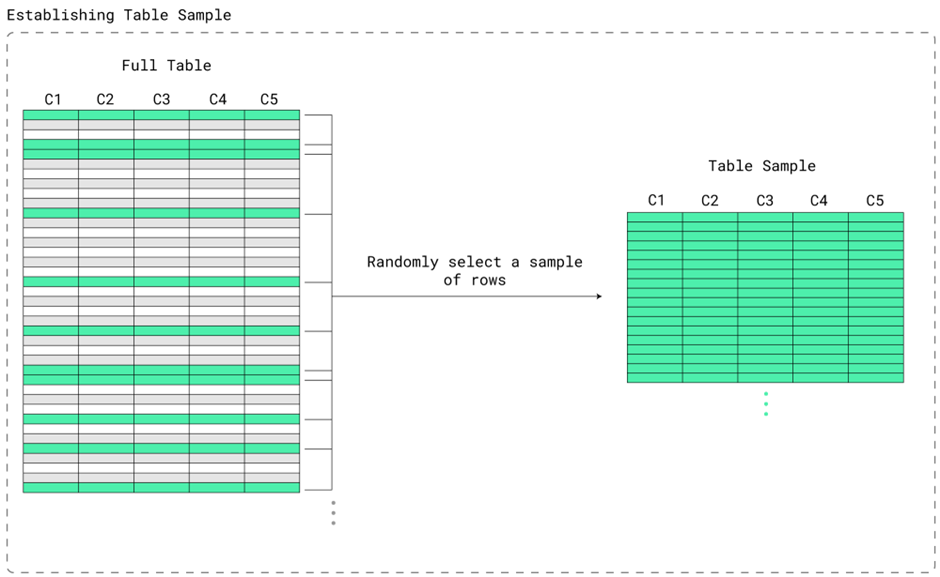
The automatic statistics collection facility has been enhanced to determine which tables do not yet contain a trained model. When such a table is found, the new model discovery component determines which columns are most appropriate to include in the model, based primarily on a correlation analysis between all columns in the table. Two or more heavily correlated columns are more likely to be included over a column that has weak or no correlation with other columns in the table. Once the desired subset of columns is determined, we are almost ready to start, but we still need some way of generating our neural network training set. Thankfully, the automatic statistics collection facility already internally collects a randomly chosen representative sample of rows from the table. This table sample is exactly what will be used to generate our neural network training set.
Training Set Generation
From the table sample, we have one or more distinct values for each column in the model. These distinct column values can then be used to generate sample predicates for the column. For example, consider the following where we have 7 samples from 5 columns of varying data types:
C1 C2 C3 C4 C5
[ ['0', '5', "Hello", 'z', '1.41'],
['42', '4', "World", 'a', '3.14'],
['222', '5', null, null, '3.14'],
['0', '5', "Hello", 'a', '1.41'],
['88', '3', "Hello", 'z', '8.88'],
['88', '3', null, 'b', '4.44'],
['500', '4', "Hello", 'c', '3.14'] ]
The sample contains 5 distinct values for the column C1 - '0', '42', '88', '222', and '500'. We can then generate a mix of potential query predicates based on these distinct values, for example an equality predicate like "C1 = 42". We can also generate range predicates, for example "C1 >= 42 AND C1 <= 88" (or equivalently "C1 BETWEEN 42 AND 88"). We have 5 columns, however our queries may specify predicates on only a subset of those columns as well. To 'ignore' a column (e.g. to represent a query that does not provide any predicates for that column), we can provide a range predicate for that column which includes all column values, for example for C1 this could be the range predicate "C1 >= 0 AND C1 <= 500". This can similarly be applied to columns that are nullable - since SQL NULL values typically sort high, we can generate 'pseudo' predicates like "C4 >= 'a' AND C4 <= null". Putting this all together, let's say we want a range predicate on C1 between 42 and 88, and a range predicate on C4 between 'a' and 'b'. Our generated query would then be:
C1 >= 42 AND C1 <= 88 and C2 >= 3 AND C2 <= 5 AND C3 >= "Hello" AND C3 <= null AND C4 >= 'a' AND C4 <= 'b' AND C5 >= 1.41 AND C5 <= 8.88
We end up generating about one million queries, where for each query we choose more-or-less randomly between a range predicate, an equality predicate, or a predicate that ignores the column, and then repeating for all other columns. The choices are not all entirely random, there is also some targeted generation of specific column predicates to expose the neural network to some special classes of common query patterns to encourage more diverse learning. We'll call these 'pseudo-queries', since they are not actual SQL queries to be executed by the database engine, rather they are a special encoding of multiple column predicates conceptually similar to SQL query predicates.
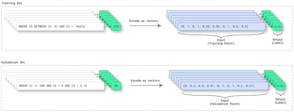
These million or so pseudo-queries will be split into 2 disjoint sets - about 90% of the pseudo-queries for the training set that will be used to train the AI Query Optimizer neural network, and about 10% of the pseudo-queries for the validation set to evaluate how well the neural network can generalize to unseen data.
Column Predicate Encoding
So far, we've seen how our training set has been generated, and the input data may be in different formats based on the column data types. However, inputs to neural networks are traditionally provided as floating point values. Conversion to floating point values is straightforward for columns containing integral or real values, and also for date/time/timestamp columns as those are typically stored using an integral data type. However, this conversion is problematic for columns containing string-based data types, or more generally any data type of an arbitrary length, where it is unclear how longer streams of bytes should best be converted into a shorter fixed-length floating point representation without (significant) loss of precision. There are various common approaches to convert string-based data types to integer or floating point representations. We won't dive into the details (input value encoding is a topic likely worthy of it's own blog post!), other than to say that the encoding approach used ensures ordering is preserved for values in that column. For example, after conversion, the string "Hello" in our example would have a smaller floating point representation than the string "World". The order-preserving characteristic is very important for the AI Query Optimizer's neural network in order to properly support input range predicates.
Even after converting all values to floating point representations, it's generally good for all inputs to a neural network to have a common scale4, for example from 0.0 to 1.0. This scaling can be done in various ways - one common way is min/max normalization, where each value subtracts the minimum value and then divides by the range of possible values (largest encoded value minus the smallest encoded value). This means the smallest encoded value would be normalized to a value of 0.0, and the largest encoded value would be normalized to a value of 1.0. This is just one possible way of scaling the encoded input values - the actual encoding and scaling approach used by the AI Query Optimizer is a little more involved, but at least this basic way of encoding and scaling can give you a good idea about how various data types can be converted into encoded scaled values suitable to input to a neural network.
Each column provides 2 input 'features' to the neural network - the column encoded minimum predicate value, and the column encoded maximum predicate value. Equality predicates from the training set pseudo-queries are converted into equivalent range predicates (e.g. 'WHERE C1 = 42' is equivalent to 'WHERE C1 >= 42 AND C1 <= 42'). In this range predicate format, the low part of the range is provided as the 'minimum' input feature to the neural network for that column, and the high part of the range is provided as the 'maximum' input feature to the neural network for that column.
Training Set Labels
So, now we know how to generate our pseudo-queries for our neural network training set, but we still need to know the training set labels so our neural network can learn. Since we want our neural network to learn to output query combined predicate selectivities, we can essentially 'evaluate' our generated training set pseudo-queries against the table sample to compute the selectivity label. For example, assuming the table sample contains 2000 samples, and a training set pseudo-query matches 3 rows from the table sample, the resulting selectivity label would be 3/2000, or 0.0015. For our sample pseudo-query above, we have a sample size of 7, and our predicates match 2 of those 7 samples, so the resulting selectivity label would be 2/7, or 0.2857. These simplified examples assume linear extrapolation from the table sample to the overall table. In cases where the AI Query Optimizer determines linear extrapolation may not be ideal, the table and/or table sample distribution information may be used to perform more advanced extrapolation computations in order to reduce selectivity estimation error.
Neural Network Training Time!
We have our training set and expected output labels, so we're ready to start training! Our training set is split into separate training and validation portions. The training portion will be used to train the neural network weights based on the expected labels, and the validation portion will be used to evaluate how well the neural network was trained. Since the two portions of the overall training set are disjoint, neural network validation is done on 'unseen' pseudo-queries, so is a good way to determine how well the neural network generalizes to unseen data.
Neural Network Architecture
The explosion of Large Language Models (LLMs) has led some experts in the field of AI to suggest 'the data is the model'. The implication is that the actual neural network architecture does not really matter too much - as long as it is large enough and there is enough clean data to learn from, any model architecture will end up performing well. Even smaller LLMs like granite.13b5 or Llama 3 8B6 have billions of parameters and can take months to train using farms of GPUs.
In comparison, even the largest AI Query Optimizer neural networks are tiny! Using the same nomenclature, the models would be named something like AIQOpt 0.00001b. There are 4 basic neural network sizes, small (~1600 parameters), medium (~3700 parameters), large (~5100 parameters), and extra large (~9600 parameters). The actual size of neural network used for a particular table depends on the number of table columns included in the model - from 2 up to 20 columns, where the chosen columns are based on model discovery as described earlier.
Even though these models are comparitively tiny, it doesn't mean they are not powerful. While LLMs are more general-purpose, the AI Query Optimizer models have a very specific, constrained task - to predict the selectivity of multiple column predicates for a single table. Having such a restricted and well-defined task as well as access to clean data (e.g. the table sample does not contain any noise) means larger models are just not necessary. This also allows for tight control on the amount of storage needed for the neural networks.
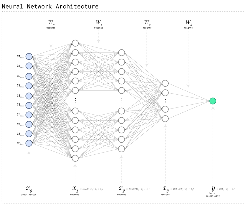
The input layer contains 2 neurons for each column in the model - one to represent the column predicate range minimum value, and one to represent the column predicate range maximum value. Besides the input layer, there are 3 fully-connected layers of various sizes, and the output layer has a size of 1 to represent the predicted selectivity. The fully-connected layers use ReLU (Rectified Linear Unit) activations to preserve input feature linearity and enable sparsity of representation for computational efficiency7. Since the combined predicate selectivity is a value between 0.0 (no rows from the table are expected to match the query) and 1.0 (all rows from the table are expected to match the query), a sigmoid activation is used for the output layer.
Neural Network Training - "Done in 60 Seconds"
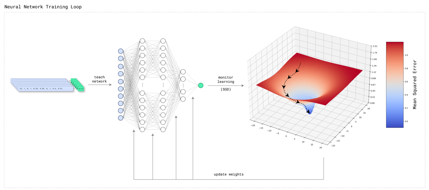
Neural network training is done using stochastic gradient descent3, combined with some custom optimizations intended to reduce training time while still providing good prediction performance. Since models are trained directly on the database system, and should ideally have minimal impact on any running database workloads, training is performed on a single CPU (the target database system may not even have any GPUs). The training time target is about 1 minute in order to minimize the model training impact on overall table statistics collection time, as well as to minimize impact on any running database workloads.
AI Query Optimizer model training may not sound impressive at first glance until you start to think about how neural networks are usually trained. The standard model training process usually involves teams of researchers and engineers spending months curating and cleansing data and then training models in isolation ahead of time, carefully validating model metrics along the way and possibly adjusting the model architecture and hyper-parameters if Neural Architecture Search didn't get everything quite right. After all this, they might finally be ready to release their model into production.
In contrast, AI Query Optimizer models are trained on production database systems, using unseen data, and trained on a single CPU in about 60 seconds. Since training is done in the background by the automatic statistics collection facility, it should also have minimal impact on your production database workload. After training, AI Query Optimizer neural networks are immediately ready to be used to improve query performance on production database systems. A massive amount of engineering work was required to make this possible. As a result of this engineering effort, neural network training happens transparently without user intervention, silently improving query performance.
Neural Network Validation
After model training is complete, the validation set is used to evaluate the performance of the model on unseen data. Although it might seem natural to think of this as validating the trained model 'accuracy', our model is a regression model (it is predicting a numerical value, the query predicate selectivity), so model validation actually involves measurement of the model error8. This also makes sense when thinking about how neural networks are trained - as the model is trained and model performance improves, the error decreases. Model validation for an AI Query Optimizer neural network then includes gathering validation metrics, which are based on the mean squared error (MSE). The MSE is the squared difference between the validation set expected labels (the query selectivities computed from the table sample) and the neural network's predictions, averaged across the entire validation set.
The validation metrics are mainly intended for diagnostic purposes, however could potentially be used for different purposes by the AI Query Optimizer in the future (e.g. if the model error is too large, a new model may be trained using a different neural network architecture, or with a larger table sample size, etc.). Most validation metrics are reported in the statistics log, which also already includes other automatic statistics collection diagnostic information. Similarly, the PD_GET_DIAG_HIST table function can also be used to query the statistics ('optstats') log to gather high-level model training information, for example to see if model discovery has been performed, as well as model training start and stop times.
The following is an example statistics log entry after model training and validation is complete:
2024-09-18-05.08.32.737152-240 I308380A2348 LEVEL: Event
PID : 56625272 TID : 12081 PROC : db2sysc 0
INSTANCE: tpcds NODE : 000 DB : BLUDB
APPHDL : 0-89 APPID: *N0.tpcds.240823011437
UOWID : 15 LAST_ACTID: 0
AUTHID : TPCDS HOSTNAME: myhost
EDUID : 12081 EDUNAME: db2agent (BLUDB) 0
FUNCTION: DB2 UDB, relation data serv, SqlrSqmlCardEstModel::trainModel, probe:200
TRAIN : TABLE CARDINALITY MODEL : Object name with schema : AT "2024-09-18-05.08.32.737152" : BY "Asynchronous" : success
OBJECT : Object name with schema, 13 bytes
TPCDS.ITEM
IMPACT : None
DATA #1 : String, 1613 bytes
Model metrics: Rating: 2 (Good), Table samples: 2000 (37565), Flags: 0x0, Training time: 69328 (23/1295/513/0), Low Bound Threshold: 0.005000, Validation MSE: 0.000072, Accuracy bucket counts: 1763,13162,38642,13172,2411, Accuracy bucket means: -3.076791,-1.345326,-0.232326,1.343618,3.454930
Table column cardinalities: 37565,34340,5,4,35969,4073,3441,953,685,17,100,11,11,1001,1021,8,34305,37565
Sample column cardinalities: 2000,1983,5,4,1976,997,813,626,546,17,100,11,11,764,755,8,1986,1992
Sample column mappings: 128,128,4,3,135,301,322,128,128,16,79,10,10,128,128,7,134,134
Column flags: 00000387,00000125,00000008,00000008,0000012D,0000150D,0000150D,0000250D,00000109,00000108,00000108,00002508,00000128,0000010D,00000109,00000008,0000012D,00000109
Base algorithm metrics: Training metric: 0.000000, Validation metric: 0.000099, Previous validation metric: 0.000069, Pre-training validation metric: 0.001802, Used training iterations: 14, Configured training iterations: 15, Training set size: 691499, Pre-training time: 2802, Training time: 27226, Accuracy bucket counts: 146,7418,31194,9038,21354, Accuracy bucket means: -2.343948,-1.260363,-0.108581,1.350975,8.149400
Low selectivity algorithm metrics: Training metric: 0.000000, Validation metric: 0.000056, Previous validation metric: 0.003615, Pre-training validation metric: 0.021132, Used training iterations: 24, Configured training iterations: 24, Training set size: 450634, Pre-training time: 2779, Training time: 42106, Accuracy bucket counts: 2454,13791,11232,14876,2708, Accuracy bucket means: -3.155077,-1.374260,0.087329,1.334569,3.600151
The following example shows model discovery ('DISCOVER') events and neural network training ('TRAIN') events from the statistics log using PD_GET_DIAG_HIST:
select substr(eventtype, 1, 9) as event, substr(objtype, 1, 23) as objtype, substr(objname_qualifier, 1, 8) as schema, substr(objname, 1, 8) as name, substr(first_eventqualifier, 1, 26) as eventtime, substr(eventstate, 1, 8) as eventstate from table(sysproc.pd_get_diag_hist ('optstats', 'ALL', 'NONE', current_timestamp - 1 year, cast(null as timestamp))) as sl where substr(objname, 1, 4) = 'ITEM' order by timestamp(varchar(substr(first_eventqualifier, 1, 26), 26))
EVENT OBJTYPE SCHEMA NAME EVENTTIME EVENTSTATE
--------- ----------------------- -------- -------- -------------------------- ----------
DISCOVER TABLE CARDINALITY MODEL TPCDS ITEM 2024-09-18-05.06.52.438883 start
DISCOVER TABLE CARDINALITY MODEL TPCDS ITEM 2024-09-18-05.07.04.713171 success
COLLECT TABLE AND INDEX STATS TPCDS ITEM 2024-09-18-05.07.04.713768 start
TRAIN TABLE CARDINALITY MODEL TPCDS ITEM 2024-09-18-05.07.23.357974 start
TRAIN TABLE CARDINALITY MODEL TPCDS ITEM 2024-09-18-05.08.32.737152 success
COLLECT TABLE AND INDEX STATS TPCDS ITEM 2024-09-18-05.08.32.756160 success
Where are Trained Models Stored?
Once the neural network has been trained and validated, it will be stored along with any other necessary metadata in a new catalog table - SYSIBM.SYSAIMODELS. The name of the model is system generated and the model is stored in a binary format, so looking at the SYSAIMODELS catalog table directly may not be too insightful. To provide more meaningful model information, a new catalog view has also been added - SYSCAT.AIOPT_TABLECARDMODELS. This catalog view allows you to see which table a model is associated with as well as which columns are included in the model. Once the neural network model (including model metadata) is stored in the SYSIBM.SYSAIMODELS catalog table, it can be used by the Db2 query optimizer.
The following is an example entry from the SYSCAT.AIOPT_TABLECARDMODELS view:
select modelschema, modelname, tabschema, tabname, substr(tabcolumns, 1, 50) as tabcolumns from syscat.aiopt_tablecardmodels where tabname = 'ITEM'
MODELSCHEMA MODELNAME TABSCHEMA TABNAME TABCOLUMNS
------------ ---------------------- ---------- -------- --------------------------------------------------
SYSIBM SQL240822215445253018 TPCDS ITEM ITEM_SK,ITEM_ID,REC_START_DATE,REC_END_DATE,ITEM_D
How are Trained Models Used During Query Compilation?
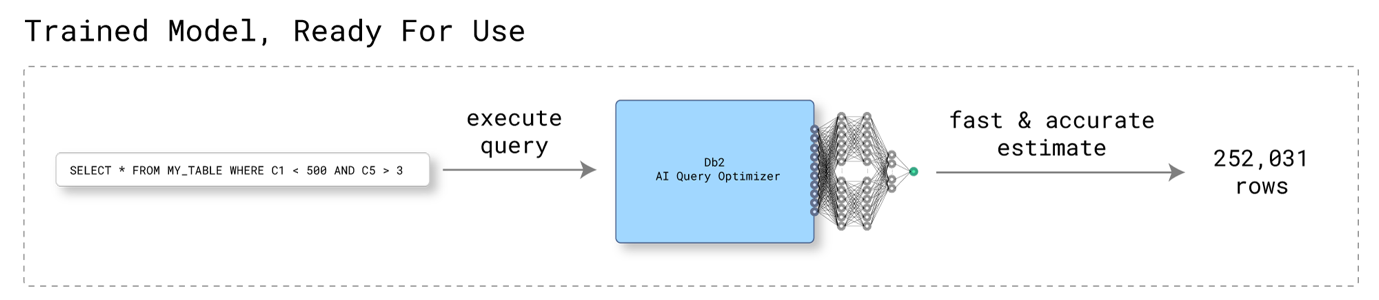
After the neural network has been trained, it can be used to help the Db2 Optimizer choose optimal access plans. If the AI Query Optimizer feature is enabled, and a trained model exists for a table involved in an SQL query, and at least some subset of the SQL query predicates can be handled by the model (e.g. equality or range predicates on 2 or more columns included in the model), the model may be used to predict the combined predicate selectivity for various query access plan alternatives being evaluated. If only a subset of the predicates can be handled by the model, the traditional statistics-based Db2 Optimizer will be used for the remaining predicates.
As a more concrete example, using a similar example as from training, let's say the query to be executed is:
SELECT * FROM MYTABLE WHERE C1 >= 42 AND C4 >= 'a' AND C4 <= 'b' AND SUBSTR(C8, 3, 20) LIKE '%AB%YZ%'
In this example, we have 2 column range predicates whose combined predicate selectivity can be predicted by the AI Query Optimizer, and 1 column (C8) that was not included in the model and so whose selectivity estimate will be managed by the traditional Db2 Optimizer. Since the range predicate upper bound was not specified for C1, the column maximum value (500) will be used as the upper bound. Since the model was trained on 3 other columns whose predicates were not specified in the query (C2, C3, C5), predicates containing the column min and max values will be used. The resulting predicates will be sent to the AI Query Optimizer for selectivity prediction:
C1 >= 42 AND C1 <= 500 and C2 >= 3 AND C2 <= 5 AND C3 >= "Hello" AND C3 <= null AND C4 >= 'a' AND C4 <= 'b' AND C5 >= 1.41 AND C5 <= 8.88
From these predicates, the AI Query Optimizer will use the trained neural network to provide a predicted selectivity for the predicates specified for columns C1 and C4, and the traditional Db2 Optimizer will use this selectivity prediction to estimate the overall query selectivity after applying any further predicates (e.g. "SUBSTR(C8, 3, 20) LIKE '%AB%YZ%'").
If you want to determine whether a model was used during query optimization, you can use the existing Db2 explain facility. The explain facility has been extended to include information detailing which predicate selectivity computations were assisted by the AI Query Optimizer.
As an example, the following formatted explain output shows a predicate whose selectivity was predicted using the neural network, indicated by the presence of a 'Filter Factor Source' (this is the name of the model for the table, as stored in the SYSIBM.SYSAIMODELS catalog table):
Predicates:
----------
3) Sargable Predicate,
Comparison Operator: Less Than or Equal (<=)
Subquery Input Required: No
Filter Factor: 0.657143
Filter Factor Source: SYSIBM.SQL240719025525017497
Predicate Text:
--------------
(Q3.COMM <= 1300)
And the following entry shows an example where a combined predicate selectivity was predicted using the neural network:
Table Cardinality Model Predicates:
-----------------------------------
Model: SYSIBM.SQL240719025525017497
Predicates:
3) (Q3.COMM <= 1300)
4) (200 <= Q3.COMM)
5) (60000 < Q3.SALARY)
6) (5 <= Q3.YEARS)
7) (Q3.JOB = 'Sales')
Summary
The Db2 AI Query Optimizer is a powerful new feature that helps Db2 determine optimal access plans for your SQL queries. Under the covers, neural networks are automatically discovered and trained as part of Db2 automatic statistics collection processing. These neural networks learn hidden data correlations, providing the Db2 Optimizer with more accurate predicate selectivity predictions. All this is done transparently and automatically, as soon as the AI Query Optimizer feature is enabled. You could continue to use your old tried-and-true statistics-based query optimizers, but wouldn't you rather upgrade now to enjoy the improved performance made available by the state-of-the-art Db2 AI Query Optimizer? Try it out today!
Image Credits
Special thanks to Nick Ostan for providing the graphics in this article to make these concepts easier to grok for visual learners, and to Malik Johnson for the title graphic.
- Zuzarte, Calisto. The AI Query Optimizer in Db2. IDUG. 2024-05-24.
- Zuzarte, Calisto & Corvinelli, Vincent. The AI Query Optimizer Features in Db2 Version 12.1. IDUG. 2024-08-12.
- Rumelhart, D. E. & Hinton, G. E. & Williams, R. J. (1986). Learning Internal Representations by Error Propagation. Parallel Distributed Processing: Explorations in the Microstructure of Cognition, Volume 1: Foundations, 318-362.
- Brownlee, Jason. How to use Data Scaling Improve Deep Learning Model Stability and Performance. Machine Learning Mastery. 2020-08-25.
- "Granite Foundation Models" (PDF). IBM. 2024-05-31.
- "Llama 3". Meta. 2024-04-18.
- Glorot, Xavier & Bordes, Antoine & Bengio, Y.. (2010). Deep Sparse Rectifier Neural Networks. Journal of Machine Learning Research. 15.
- Brownlee, Jason. Regression Metrics for Machine Learning. Machine Learning Mastery. 2021-02-16.
Liam joined IBM in 1999 as a software developer, and since then has been designing and implementing various features in Db2 LUW. Most recently, Liam has been leading the Machine Learning Infrastructure area for the Db2 AI Query Optimizer.